Belief manifolds, and how to steer along them

“Nature, to be commanded, must be obeyed.”

— Francis Bacon, Novum Organum I.3 (1620)

Introduction

I believe that a deep understanding of how AI systems work internally will be crucial for medium and long term AI safety.

Why? Because to mitigate the risks of a system, you must understand it.¹

So, for my BlueDot Technical AI Safety Project, I wanted to get more familiar with an emerging paradigm in mechanistic interpretability that I think will be particularly important: the intrinsic geometry of representations in LLMs.

To that end, I decided to reproduce a research paper on this topic from the team at Goodfire: “The Shape of Beliefs: Geometry, Dynamics, and Interventions along Representation Manifolds of Language Models’ Posteriors” by Sarfati et al. (2026).

Why does this work matter?

Better steering by respecting the geometry of representations

The linear representation hypothesis (LRH) proposes that concepts or features are represented by linear directions in activation space. This approach has been highly successful, as simple linear probes can be very powerful (Chen et al., 2025; Lindsey et al., 2026). But recently, there has been what I’ll call a ‘geometric turn’ in mechanistic interpretability, which can be understood as a generalization of the LRH.

Under the geometric paradigm, instead of decoding single directions that represent features, researchers aim to study manifolds of activations: low-dimensional subspaces embedded in activation space, potentially with non-Euclidean geometry—i.e., curvature (see Engels et al., 2024; Park et al., 2024; Modell et al., 2025; Gurnee et al., 2026; Feucht et al., 2026; Fel et al., 2026; Wollschläger et al., 2026; Bhalla et al., 2026).

This mirrors earlier developments in computational neuroscience, which has undergone a similar geometric turn over the past couple of decades. As improving technology has allowed recording from ever larger numbers of neurons, the goal of analysis has shifted from understanding single-neuron activity to understanding the dynamics of neural populations (Churchland et al., 2012; Gallego et al., 2017; Chung et al., 2018; Allen et al., 2019; Gründemann et al., 2019; Stringer et al., 2019; Stringer et al., 2019; Jazayeri & Ostojic, 2021; Beshkov et al., 2024). In fact, I think there are important lessons that mechanistic interpretability can take from neuroscience here, which I discuss in connection with some of my own research that used high-throughput calcium imaging to study population activity in the mouse visual cortex (see Decodability is not function).

One concrete promise of the geometric approach is that by respecting the intrinsic structure of the model’s representations, activation steering can be done more precisely and with fewer unintended effects. This has natural applications to AI control, e.g., removing unsafe or undesirable tendencies while maintaining capabilities, by steering along the manifold that represents the feature(s) of interest.

The shape of beliefs

Sarfati et al. (2026) demonstrated this in an elegant study. Using a toy scenario as a proof of principle, they uncover what they term belief manifolds: curved subspaces of the model’s in-context posterior estimates about properties of the input—in this case, representations of the mean and variance of the distribution of a series of integers, which inform and shape its predictions for the next token. They then show that manifold-aware steering can manipulate the model’s posterior estimate of the mean without affecting its estimate of the variance (within a certain regime of values), a preliminary indication that this application of the geometric perspective above holds promise.

For this project, I set out to reproduce their results. And I was successful! (With one minor exception; see Appendix.)

After describing the reproduction, I discuss one of the most interesting points in the paper: the distinction between primal and dual representations, i.e., between the manifold structure of activations and how features are read out from them. This connects to a long-running debate in systems neuroscience over whether ‘encoding’ is the right metaphor for understanding neural activity (Brette, 2019; Buzsáki, 2019; see Decodability is not function). Then I briefly sketch a few possible extensions. The one I’m most interested in is whether this approach can be used to detect and steer evaluation awareness, i.e., the model’s belief about whether it is currently being tested, an important concern in alignment research (Laine et al., 2024; Nguyen et al., 2025; see Possible Extensions).

Update: Recently, the team at Goodfire has been pushing hard in this direction!² Shortly after I began this project, they published several new studies on neural geometry (Wurgaft et al., 2026; Geiger et al., 2026; Feucht et al., 2026). I’m excited to see so much rapid progress with this approach, and looking forward to seeing how far the field can take it.

Second Update: And then just today (May 21, 2026), Goodfire published another study showing how SAE features tile manifolds! (Bhalla et al., 2026) They are really on fire 🔥

Reproduction

Sarfati et al.’s setup is a controlled in-context learning task. The model is Llama 3.2 1B, prompted with a comma-separated sequence of integers drawn from $\mathcal{N}(\mu, \sigma)$; its next-number logits, treated as a distribution over the integer tokens, serve as its in-context posterior over the generating distribution. By sweeping $(\mu, \sigma)$ across a grid, or switching mid-sequence, Sarfati et al. investigate how the model updates its posterior over the distribution parameters and study the geometry, dynamics, and steerability of the corresponding internal representations. Unless noted, analyses are on the residual stream at layer 15.

Geometry

Belief manifolds

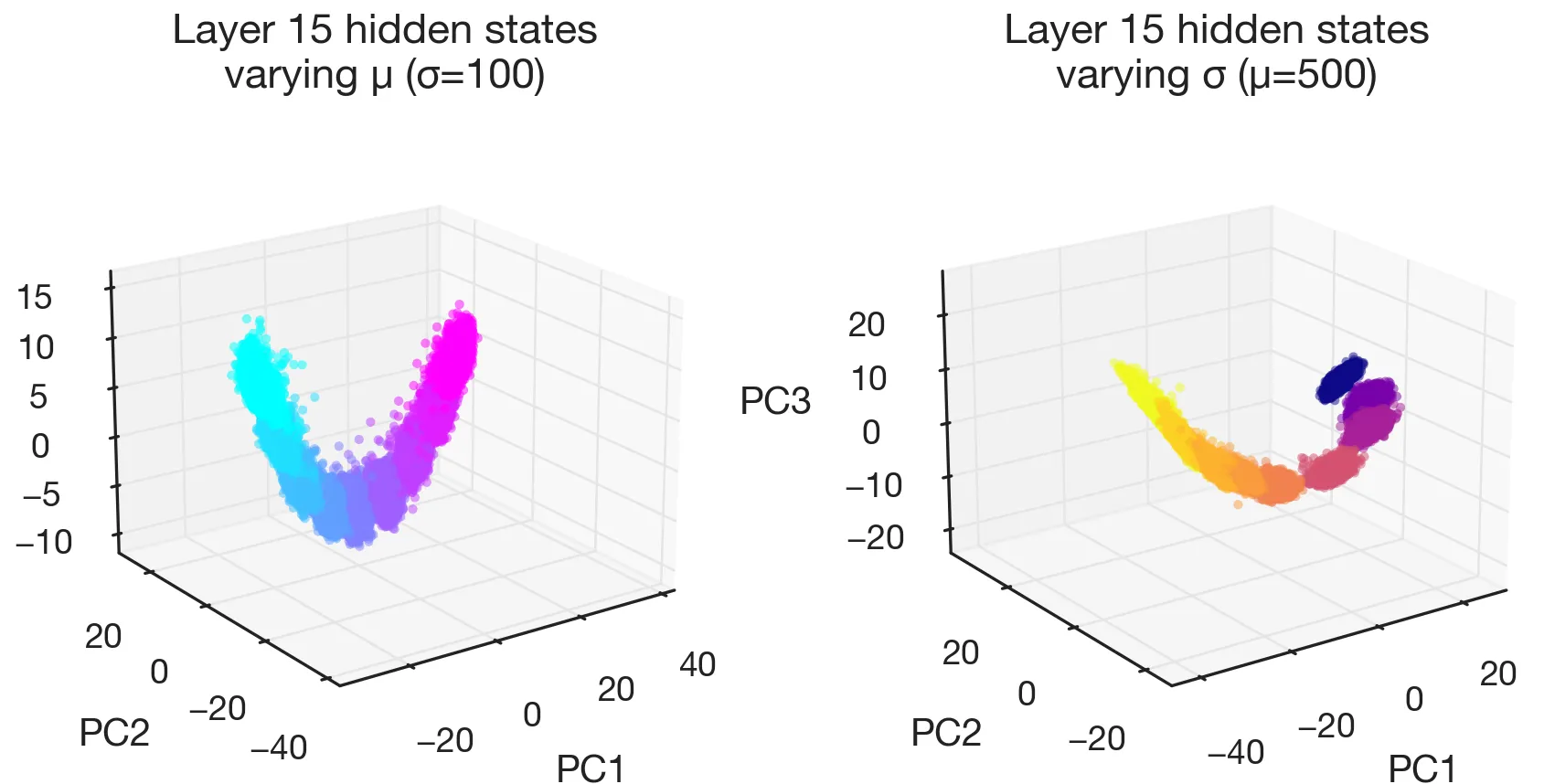
Holding $\sigma$ fixed and sweeping $\mu$ traces out a curved one-dimensional manifold in activation space; holding $\mu$ fixed and sweeping $\sigma$ traces out a second, roughly orthogonal one. These are the manifolds of the model’s beliefs about the input statistics, i.e., in-context posterior estimates of the distribution parameters (here, after it sees 500 number tokens).

Output distributions

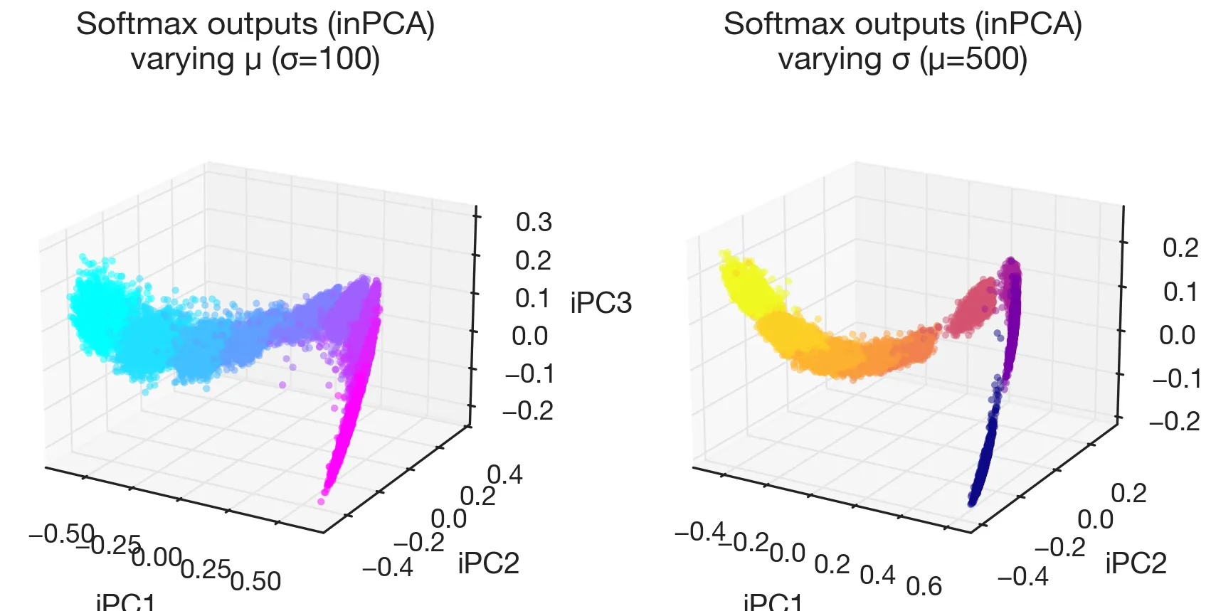
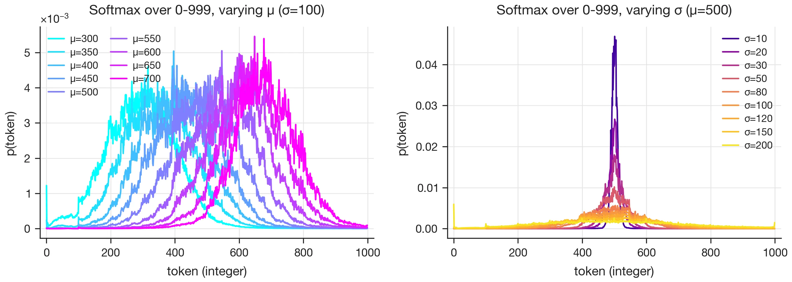
The same curved structure shows up on the output side: embedding the softmax distributions via inPCA (a variant of PCA suited to probability vectors) yields manifolds that mirror the hidden activation manifolds, and projecting the softmax onto the integer tokens 0–999 directly shows that each output distribution is approximately Gaussian with the right mean and variance.

Linear field probes

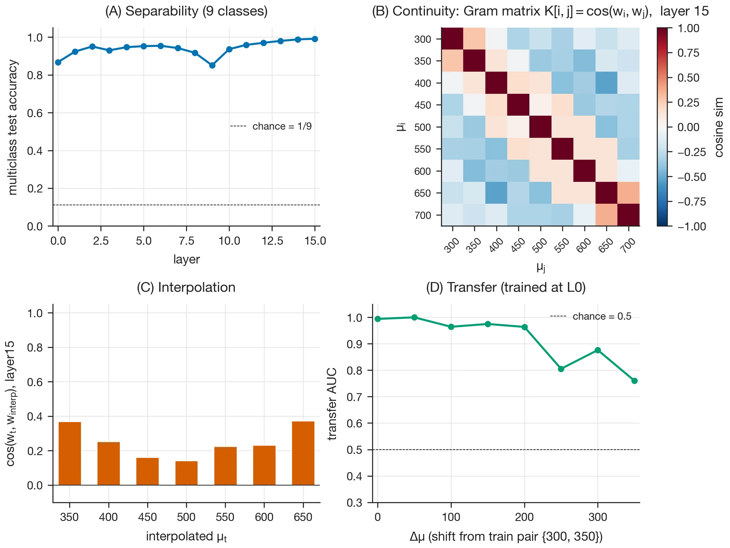
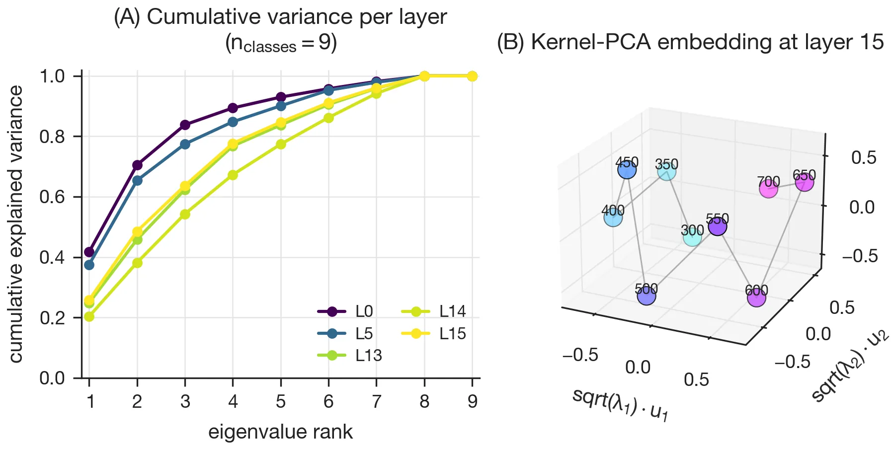
The properties that define a field of linear probes that tile the manifold (Yocum et al., 2025) are (A) high separability across all layers, (B) smooth variation of the probe directions with the feature of interest, (C) smooth interpolation of the probe vectors between trained values, and (D) local-only transfer between nearby values.

In Fig. 4, a multiclass $\mu$-probe trained at each layer recovered these qualitative properties. However, the one part that I could not reproduce quantitatively is the interpolation magnitudes in the paper’s Fig. 3C.

To investigate this, I tried a systematic sweep over the method variants described in the paper’s appendix (different probe parameterizations, optimizers, and interpolation schemes), but this did not reveal the issue. I then tried running the authors’ own released code end-to-end in case there was an error in my implementation, but the kernel-interpolation cosines still came out below the reported values.

So the qualitative claim that the probes form a coherent field rather than a set of unrelated classifiers still holds, but the published magnitudes were not reproducible, even with the authors’ code. I elaborate on this attempt in the Appendix.

Field geometry

The cumulative eigenspectrum of the probe Gram matrix shows the intrinsic dimensionality of the field rising through the network and then dropping sharply at the final layer (the so-called “late-layer anomaly.”) I could reproduce this, but it turns out to be optimizer-dependent: training the same probes with L-BFGS instead of AdamW removes the late-layer dip and yields low intrinsic dimensionality at every layer (see Appendix). Whatever the late-layer anomaly corresponds to, it appears to be at least partly a property of how the probes are fit, not solely of the representations themselves.

Dynamics

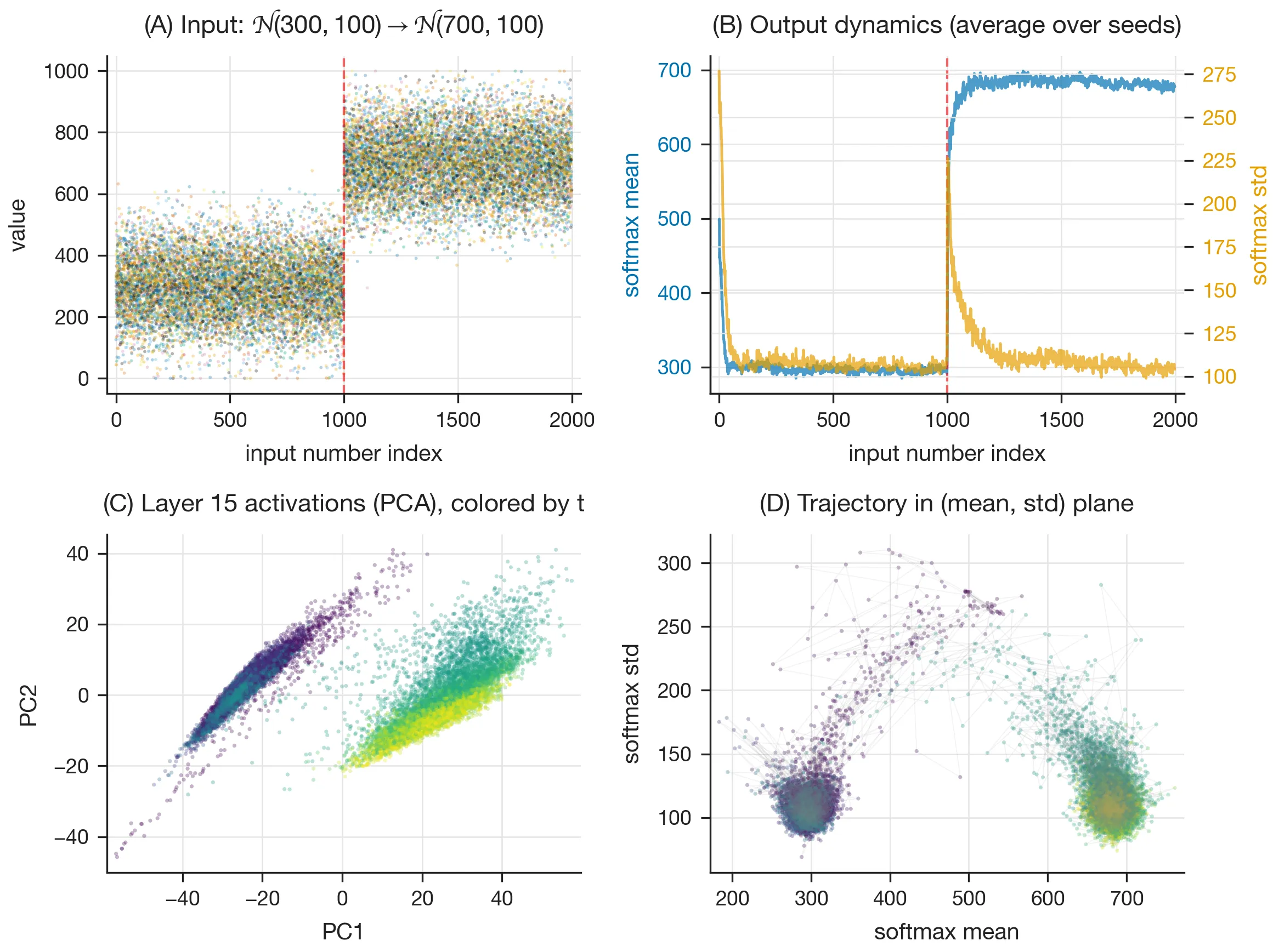
Switching distributions. When the generating distribution is changed mid-sequence from $\mathcal{N}(300, 100)$ to $\mathcal{N}(700, 100)$ (Fig. 6A), the model in-context learns the new input statistics (B), reflected in the activation trajectory (C) and the output statistics (D).

Interventions

Manifold-aware steering in the primal space (data manifold of activations)

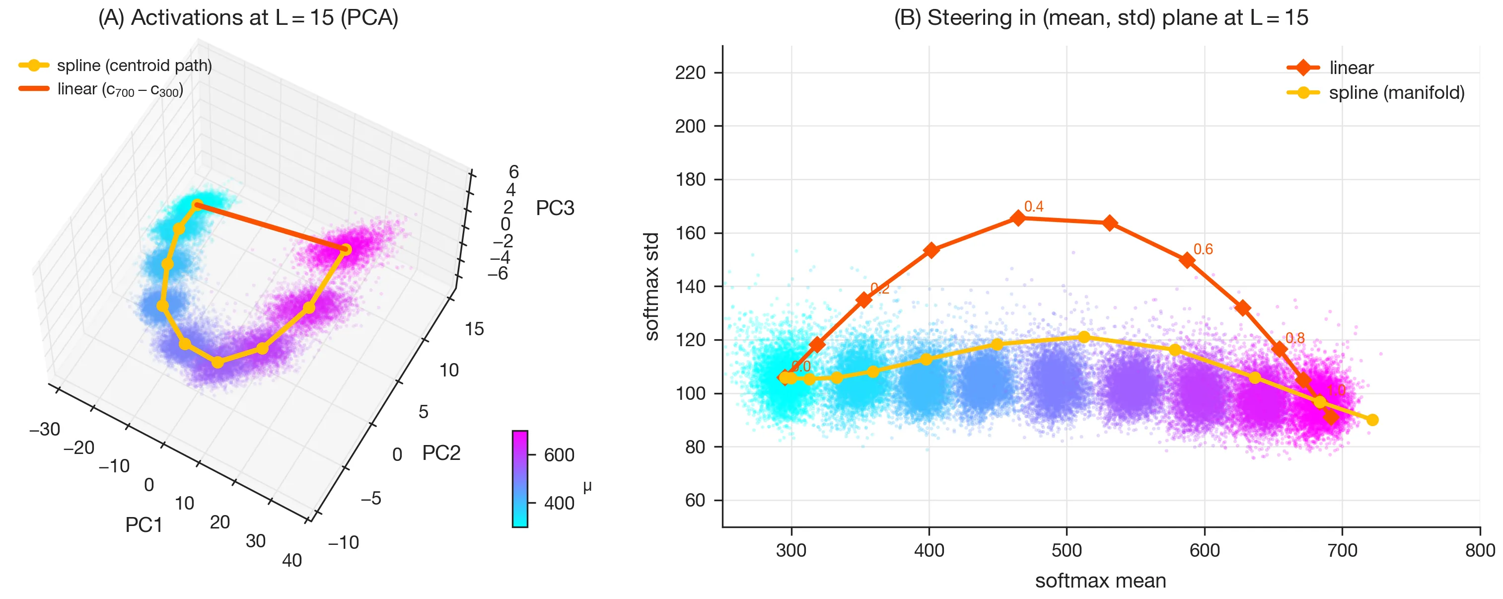
Linear steering along the vector from $\mu = 300$ to $\mu = 700$ (Fig. 7A, red line) pushes the model’s output distribution off the underlying manifold: the variance increases as the mean is changed, just as the paper reports (Fig. 7B, red curve).

By contrast, if we instead respect the belief geometry and steer along the path in activation space defined by the centroids of the mean estimates (Fig. 7A, yellow spline), the model’s belief about the mean is changed without significantly affecting its belief about the variance (Fig. 7B, yellow curve).

This demonstrates the utility of manifold-aware steering in the primal space (the data manifold of activations).

Manifold-aware steering in the dual space (field of linear features)

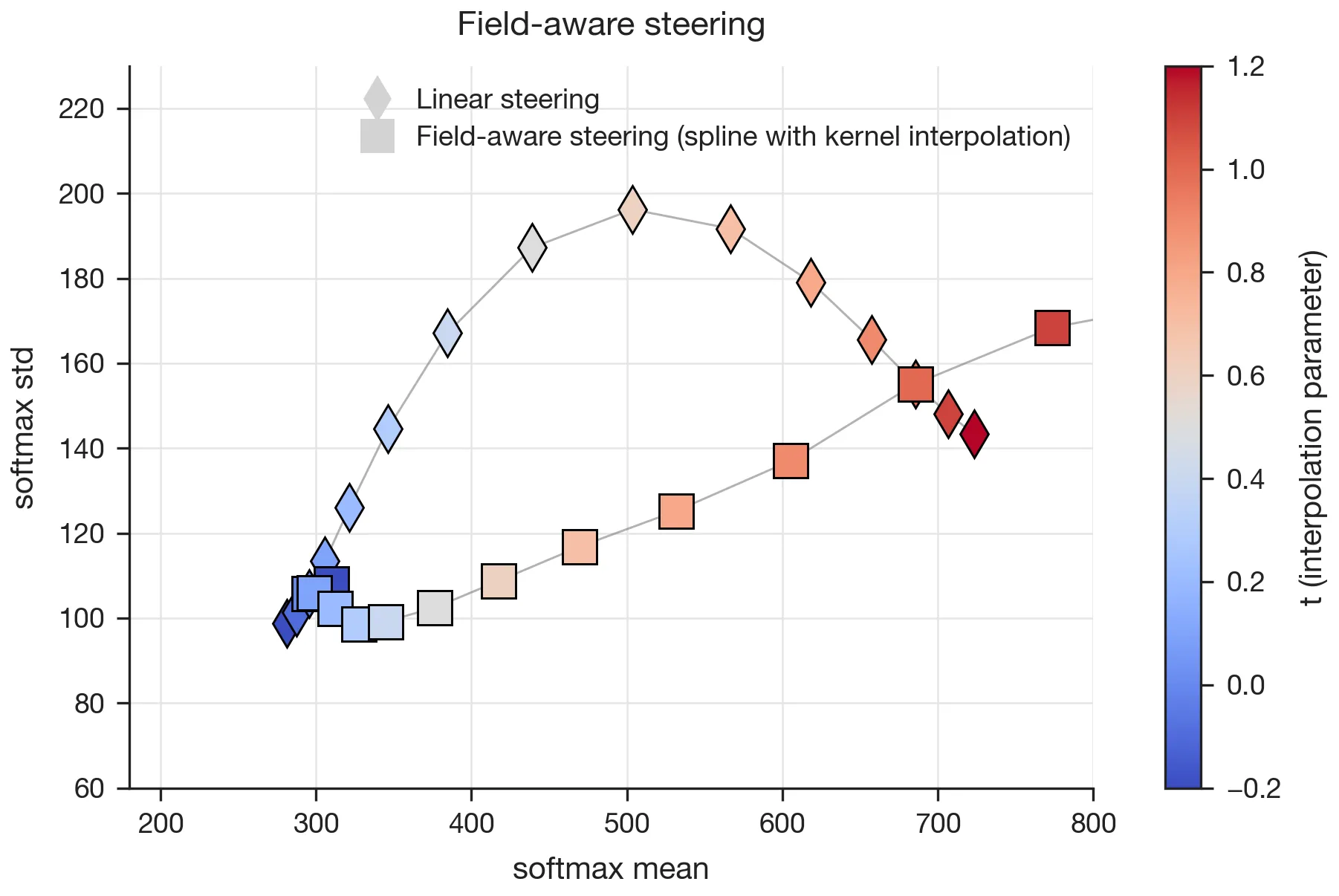
Manifold-aware steering also works in the dual space defined by the linear field probes. As with the primal space approach, steering along an LFP-derived direction that respects the smooth structure of the probe field preserves $\sigma$ across a substantial $\mu$ range (Fig. 8).

It is not clear from the paper exactly which method was used. Here, I used the kernel-interpolation approach described in Appendix D.3: at each target $\mu$ I solve $a(\mu) = K^{-1} k(\mu)$ for the Gram-regression weights and build the interpolated probe $\tilde{w}(\mu) = W_n^\top a(\mu)$, where $W_n$ is the centered, row-normalized matrix of probe weights and $w_{300}$ is its row at $\mu = 300$. The steered activation is then $x + \alpha \cdot (\tilde{w}(\mu) - w_{300})$, where I factor the steering scalar as $\alpha = t \cdot \kappa$ so that $t \in [0, 1]$ parametrizes the interpolation as $\mu(t) = 300 + 400 t$ ($t=0$ recovers the start probe and $t=1$ the end probe), and $\kappa$ is a magnitude scalar.

Now, as Sarfati et al. mention in the paper, “feature geometry is agnostic to scale”, and as far as I can tell, they combined $t$ and $\kappa$ into a single scalar $\alpha$. I decoupled them so the two effects could be studied independently. I set $\kappa = 29$ so that the path-endpoint displacement matches the natural centroid-chord magnitude of the data-manifold approach in Fig. 7. With this calibration, the spline trajectory increases $\mu$ while holding $\sigma$ relatively steady across $\mu = 300\text{–}500$, while the naive linear steering at the same $\alpha$ pushes the activations off the field manifold and increases $\sigma$.³

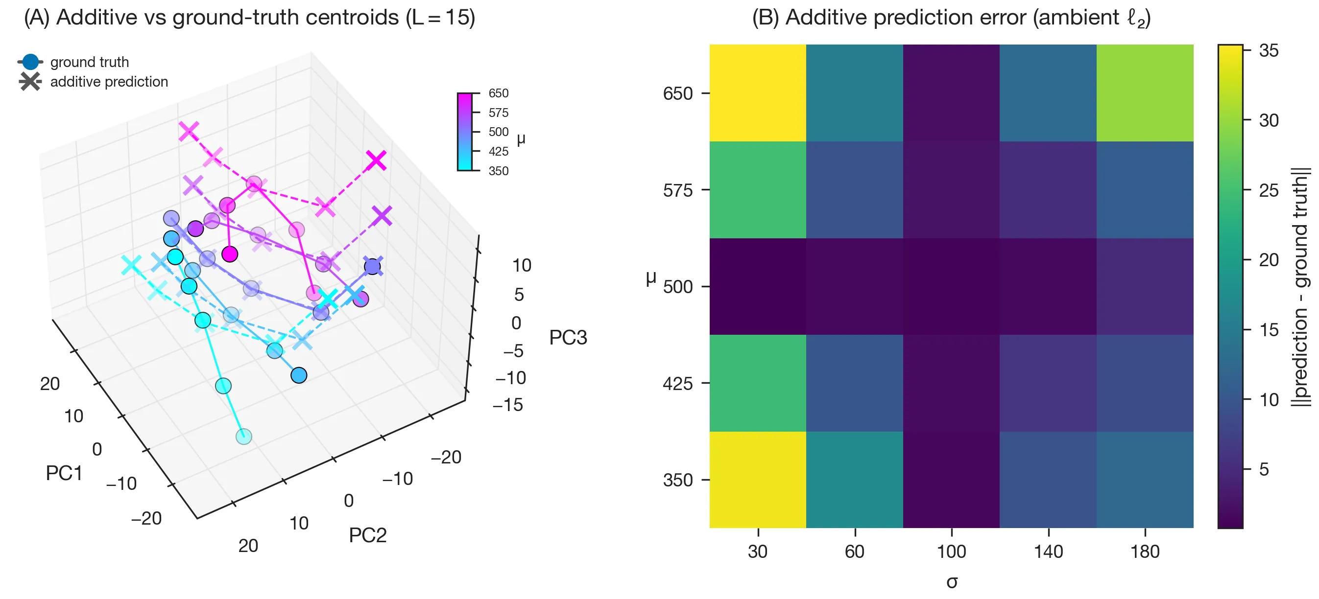
Mixture of manifolds. Finally, Sarfati et al. ask whether the joint $(\mu, \sigma)$ manifold decomposes additively as a sum of a $\mu$-spline and a $\sigma$-spline, anchored at $(\mu_0, \sigma_0) = (500, 100)$. Fitting this decomposition and comparing to the ground-truth grid of $(\mu, \sigma)$ centroids, the interpolation matches near the anchor and degrades at the corners. This indicates that $\mu$ and $\sigma$ interact non-linearly in the embedding: the joint manifold doesn’t factor cleanly into additive contributions, reproducing the paper’s negative result.

Discussion

Decodability is not function

One of the most compelling theoretical points in the paper is the distinction between primal and dual representations. This is a key idea in information geometry, a beautiful area of math pioneered by Shun-ichi Amari that weds probability and statistics with differential geometry. In this case, a point in the primal space is a particular concrete activation in the model’s residual stream. A point in the dual space is a weight vector of a linear probe: a direction that you can project activations onto to distinguish a given feature (here, the mean).

Each of these gives a different way of looking at the model’s posterior belief about the input distribution: the data manifold of activations (Fig. 1) and the field manifold of linear probes that tile the data manifold. The difference between the two is nicely illustrated in Sarfati et al.’s Figure 12, Appendix D.1. This is a generalization of the LRH: a feature is not a direction, it’s a field of directions, indexed by feature value. Linear separability is a property of the dual space; the curvature of the data manifold is a property of the representation in primal space. The two spaces are related, but neither constrains the other: a probe can identify a feature with near-perfect accuracy and yet point in a direction that doesn’t follow the geometry of the model’s own representational manifold.

This difference has an important operational consequence, apparent in Fig. 7 and Fig. 8. Naive linear steering along the vector pointing from the $\mu = 300$ centroid to the $\mu = 700$ centroid—a direction that separates $\mu = 300$ from $\mu = 700$ in the dual sense—pushes the activation off the belief manifold, simultaneously increasing $\sigma$ as it changes $\mu$. By contrast, manifold-aware steering changes $\mu$ while keeping $\sigma$ relatively stable—whether along the primal belief manifold (Fig. 7B, yellow curve) or along the dual-space probe field (Fig. 8, squares), i.e., the kernel-interpolated probe direction. So we see that steering that follows the model’s intrinsic activation geometry, i.e., its representational structure, is able to more precisely manipulate the model’s beliefs. A key reason for this is that a linear probe tells you only what is linearly decodable from the activations; it does not imply that direction is functionally relevant to the model.

This connects to a long-running debate in systems neuroscience, which has been wrestling with this distinction since the advent of decoding methods. Neuroscientists such as Brette (2019) and Buzsáki (2019) have argued that the standard story that ‘the brain encodes external variables to be decoded by downstream readers’ is at best a useful metaphor, and at worst actively misleading. The brain is an internally-driven dynamical system, and the fact that some external variable is linearly decodable from a neural population does not mean that it is functionally relevant to the system. Along these lines, my own prior work using calcium imaging in mouse V1 attempted to characterize population activity in terms of its intrinsic structure rather than purely its decodable content (Mayner et al., 2022). I showed that an intrinsic measure of the ‘differentiation’ of neural activity dissociates from decoding accuracy, and unlike decoding approaches, our measure pointed towards specific layers of cortex as representing differences between natural and artificial stimuli.

In interpretability research, we are fortunate because it’s easy to causally intervene. In a model, unlike in real brains, you can just perturb the population activity and see what happens. That means it is much more feasible to establish what does functionally matter for the system. The manifold-aware steering approach operationalizes this ‘decodability vs. function’ distinction; by respecting the geometry of the model’s representation, you can steer the model better.

Possible extensions

Eval awareness. One area I would like to pursue is whether this can be applied to eval awareness. This is an important issue in alignment research, and linear steering has been applied to it (Nguyen et al., 2025). Is there a curved manifold of the model’s belief about whether it is currently being evaluated, and can we use manifold-aware steering to reduce eval awareness without unintentionally affecting other beliefs or behaviors?

Minkowski-sum representations. Sarfati et al. attempted to decompose the ($\mu, \sigma$) sheet as a product manifold of independent subspaces in additive superposition, using spline-based interpolated centroids. As seen in Fig. 9, this did not work. They point to an alternative decomposition suggested by Fel et al. (2026), who proposed the Minkowski Representation Hypothesis, in which representations are Minkowski sums of convex concept polytopes (rather than vector sums of points/directions). Testing whether the ($\mu, \sigma$) manifold can be recovered as a Minkowski sum of convex hulls of activations would be an interesting follow-up analysis.

Higher-dimensional manifolds. A natural extension would be to increase the dimensionality of the task, i.e., change the setup so that the belief manifold has intrinsically $n$-dimensional structure for $n > 2$.

More abstract beliefs. Sarfati et al. raise this explicitly in the paper: their setup is a toy model of belief manifolds that relies on a numerical setting with continuous parametrizations, and it remains to be seen if the approach can generalize to more abstract natural language settings.

Conclusion

The geometric structure of internal representations in LLMs is striking because it is not guaranteed to emerge. A priori, the model’s internal representations need not lie on low-dimensional smooth manifolds, yet there’s increasing evidence that this is common. And, even better, it can be leveraged for more precise model steering.

The fact that this representational geometry does emerge as a computational motif points to a potentially very deep property of how AIs learn the structure of the world. I’m curious whether this can ultimately be formalized and explained as part of the recently proposed ‘scientific theory of deep learning’ (Simon et al., 2026). If so, that would be good news for AI safety!

Finally, I want to note that at the abstract level of representation geometry, there may be deep correspondences between how biological and artificial neural networks learn and shape their dynamics. Further cross-pollination between neuroscience and interpretability research could help uncover those connections.

Acknowledgements

Thanks to BlueDot Impact for providing such an effective way to quickly get oriented and involved in the field of AI safety.

I also want to thank the wonderful BlueDot facilitators I’ve worked with, Sandy Tanwisuth, Jess Bergs, and Katarina Slama, for their support and advice.

And, of course, thanks to Sarfati et al. and the rest of the team at Goodfire for doing this cool work!

I used Claude Code for assistance with coding and editing.

Appendix

Investigating the Fig. 3C interpolation magnitudes

The discrepancy in Fig. 3C is large enough that it can’t be explained by seed variance or a implementation detail (paper cosines of roughly $0.55$–$0.85$ vs. mine of roughly $-0.05$–$0.4$). I made two attempts to investigate this.

Sweeping probe and interpolation variants. First, I systematically swept the variants given in the paper’s appendix: multiclass vs. one-vs-rest probes, centered vs. raw weights, bias on vs. off, layer 14 vs. layer 15, single-seed vs. 5-seed-averaged probes, and all four interpolation schemes the paper describes: linear, geodesic, kernel-Gram at a range of $\lambda$ regularization values, and eigenbasis (Yocum et al., 2025). For the eigenbasis method I used kernel-PCA coordinates $\varphi(\mu_i) = \sqrt{\lambda_\beta}\,v_\beta[i]$, per-component linear interpolation at the target $\mu$, back-projection via the dual basis $u_\beta = W_n^\top v_\beta / \sqrt{\lambda_\beta}$. The best configuration I found was eigenbasis interpolation with rank-3 truncation on a multiclass probe at layer 15 (raw and centered weights gave very similar mean cosines, $\sim 0.36$), but this was still short of the paper’s $\sim 0.70$.

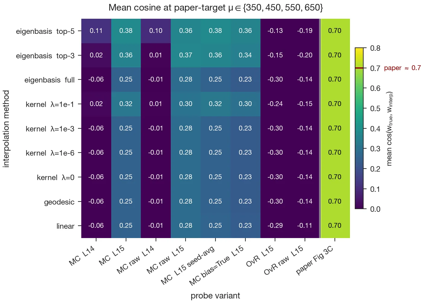
Running the authors’ released code. Second, assuming that I’d made a mistake in the implementation, I ran the authors’ own code from their public repo. The probes themselves are essentially identical to mine; test accuracy is within $0.01$ of the paper’s reported value, and the Gram-matrix top-3 eigenvalue fraction matches theirs. But I still got the same range of interpolation cosines. My best guess is that some element of the pipeline is missing from the repo.

The “late-layer anomaly” is optimizer-dependent

Sarfati et al. trained their probes with AdamW and weight decay, and reported that the intrinsic dimensionality of the field (as measured by the top-eigenvalue fraction of the Gram matrix) increases across layers and then decreases at the final layer. I found this phenomenon to be sensitive to training hyperparameters, which made me wonder if it was an optimization artifact instead of a property of the representations.

To test this, I retrained the same probes with L-BFGS, a second-order optimizer that converges to a sharper minimum of the cross-entropy loss. With L-BFGS, the top-3 cumulative variance fraction is high at every layer ($\sim0.84$), including the final one: the “late-layer anomaly” disappears, and the field appears to be low-dimensional throughout. One caveat is that this reversal requires using no feature scaling and no bias, matching the paper’s setup. Including StandardScaler in the L-BFGS pipeline partially restores the anomaly (top-3 fraction decreases to $\sim0.67$ at L14), because feature scaling reshapes the regularisation landscape enough to change the character of the solution. So the anomaly is not invariant to all reasonable optimizer choices, but the apples-to-apples comparison with the setup described in the paper does extinguish it, meaning that in that case it’s due to the AdamW optimizer rather than a fixed property of the representations. This doesn’t mean the late-layer geometry is identical to that of the earlier layers, but the intrinsic dimensionality given in the paper is at least partly an artifact of how the probes are fit.

References

- Chen, R., Arditi, A., Sleight, H., Evans, O., & Lindsey, J. (2025). Persona Vectors: Monitoring and Controlling Character Traits in Language Models. arXiv:2507.21509.
- Lindsey, J., et al. (2026). Emotion Concepts and their Function in a Large Language Model. Transformer Circuits Thread, April 2026.
- Engels, J., Michaud, E. J., Liao, I., Gurnee, W., & Tegmark, M. (2024). Not All Language Model Features Are One-Dimensionally Linear. arXiv:2405.14860.
- Gurnee, W., Ameisen, E., Kauvar, I., Tarng, J., Pearce, A., Olah, C., & Batson, J. (2026). When Models Manipulate Manifolds: The Geometry of a Counting Task. arXiv:2601.04480. (Companion: Transformer Circuits Thread.)
- Feucht, S., Lubana, E. S., Haklay, T., Fel, T., Bhalla, U., Geiger, A., Wurgaft, D., Rager, C., Sarfati, R., Merullo, J., McGrath, T., & Lewis, O. (2026). A Geometric Calculator Inside a Neural Network. arXiv:2605.01148. (Companion blog post: A Geometric Calculator Inside a Neural Network.)
- Park, K., Choe, Y. J., Jiang, Y., & Veitch, V. (2024). The Geometry of Categorical and Hierarchical Concepts in Large Language Models. arXiv:2406.01506.
- Modell, A., Rubin-Delanchy, P., & Whiteley, N. (2025). The Origins of Representation Manifolds in Large Language Models. arXiv:2505.18235.
- Fel, T., Wang, B., Lepori, M. A., Kowal, M., Lee, A., Balestriero, R., Joseph, S., Lubana, E. S., Konkle, T., Ba, D., & Wattenberg, M. (2026). Into the Rabbit Hull: From Task-Relevant Concepts in DINO to Minkowski Geometry. arXiv:2510.08638.
- Wollschläger, T., Elstner, J., Geisler, S., Cohen-Addad, V., Günnemann, S., & Gasteiger, J. (2026). The Geometry of Refusal in Large Language Models: Concept Cones and Representational Independence. arXiv:2502.17420.
- Churchland, M. M., Cunningham, J. P., Kaufman, M. T., Foster, J. D., Nuyujukian, P., Ryu, S. I., & Shenoy, K. V. (2012). Neural population dynamics during reaching. Nature, 487(7405), 51–56.
- Gallego, J. A., Perich, M. G., Miller, L. E., & Solla, S. A. (2017). Neural Manifolds for the Control of Movement. Neuron, 94(5), 978–984.
- Chung, S., Lee, D. D., & Sompolinsky, H. (2018). Classification and Geometry of General Perceptual Manifolds. Physical Review X, 8(3), 031003.
- Allen, W. E., Chen, M. Z., Pichamoorthy, N., Tien, R. H., Pachitariu, M., Luo, L., & Deisseroth, K. (2019). Thirst regulates motivated behavior through modulation of brainwide neural population dynamics. Science, 364(6437), eaav3932.
- Gründemann, J., Bitterman, Y., Lu, T., Krabbe, S., Grewe, B. F., Schnitzer, M. J., & Lüthi, A. (2019). Amygdala ensembles encode behavioral states. Science, 364(6437), eaav8736.
- Stringer, C., Pachitariu, M., Steinmetz, N., Reddy, C. B., Carandini, M., & Harris, K. D. (2019). Spontaneous behaviors drive multidimensional, brainwide activity. Science, 364(6437), eaav7893.
- Stringer, C., Pachitariu, M., Steinmetz, N., Carandini, M., & Harris, K. D. (2019). High-dimensional geometry of population responses in visual cortex. Nature 571, 361–365.
- Jazayeri, M., & Ostojic, S. (2021). Interpreting neural computations by examining intrinsic and embedding dimensionality of neural activity. Current Opinion in Neurobiology, 70, 113–120.
- Beshkov, K., Fyhn, M., Hafting, T., & Einevoll, G. T. (2024). Topological structure of population activity in mouse visual cortex encodes densely sampled stimulus rotations. iScience, 27(4), 109370.
- Sarfati, R., Bigelow, E., Wurgaft, D., Merullo, J., Geiger, A., Lewis, O., McGrath, T., & Lubana, E. S. (2026). The Shape of Beliefs: Geometry, Dynamics, and Interventions along Representation Manifolds of Language Models’ Posteriors. arXiv:2602.02315.
- Laine, R., Chughtai, B., Betley, J., Hariharan, K., Scheurer, J., Balesni, M., Hobbhahn, M., Meinke, A., & Evans, O. (2024). Me, Myself, and AI: The Situational Awareness Dataset (SAD) for LLMs. arXiv:2407.04694.
- Wurgaft, D., Goodman, N. D., Rager, C., Fel, T., Kowal, M., Geiger, A., Shyam, V., Lubana, E. S., Feucht, S., Bhalla, U., Haklay, T., Bigelow, E., Sarfati, R., McGrath, T., Lewis, O., & Merullo, J. (2026). Manifold Steering Reveals the Shared Geometry of Neural Network Representation and Behavior. arXiv:2605.05115. (Companion blog post: Steering Along Manifolds to Control Neural Networks.)
- Geiger, A., Lubana, E. S., Fel, T., Merullo, J., Byun, M. J., Lewis, O., & McGrath, T. (2026). The World Inside Neural Networks. Goodfire Research, May 2026.
- Brette, R. (2019). Is coding a relevant metaphor for the brain? Behavioral and Brain Sciences, 42, e215.
- Buzsáki, G. (2019). The Brain from Inside Out. Oxford University Press.
- Mayner, W. G. P., Marshall, W., Billeh, Y. N., Gandhi, S. R., Caldejon, S., Cho, A., Griffin, F., Hancock, N., Lambert, S., Lee, E. K., Luviano, J. A., Mace, K., Nayan, C., Nguyen, T. V., North, K., Seid, S., Williford, A., Cirelli, C., Groblewski, P. A., Lecoq, J., Tononi, G., Koch, C., & Arkhipov, A. (2022). Measuring Stimulus-Evoked Neurophysiological Differentiation in Distinct Populations of Neurons in Mouse Visual Cortex. eNeuro, 9(1), ENEURO.0280-21.2021. DOI: 10.1523/ENEURO.0280-21.2021.
- Nguyen, J., Hoang, K., Attubato, C. L., & Hofstätter, F. (2025). Probing and Steering Evaluation Awareness of Language Models. arXiv:2507.01786.
- Simon, J., Kunin, D., Atanasov, A., Boix-Adserà, E., Bordelon, B., Cohen, J., Ghosh, N., Guth, F., Jacot, A., Kamb, M., Karkada, D., Michaud, E. J., Ottlik, B., & Turnbull, J. (2026). There Will Be a Scientific Theory of Deep Learning. arXiv:2604.21691.
- Yocum, J., Allen, B., Olshausen, B. A., & Russell, S. (2025). Neural Manifold Geometry Encodes Feature Fields.
- Bhalla, U., Fel, T., Rager, C., Feucht, S., Haklay, T., Wurgaft, D., Boppana, S., Kowal, M., Shyam, V., Merullo, J., Geiger, A., & Lubana, E. S. (2026). Do Sparse Autoencoders Capture Concept Manifolds? arXiv:2604.28119.